Before we describe what Batch Normalisation is, here are a few introductory terms
Internal covariate shift
Stochastic Gradient Descent uses a minibatch of input to train the parameters of a layer. The input to a layer is the output from the previous layer. A change in the parameters of the previous layer causes a change in the distribution of the input to the current layer and this causes problems in convergence since the parameters in the current layer have to continuously change to adapt to the changing input distribution. The change in distributions of internal nodes of a deep network is known as the internal covariant shift.
Batch Normalising transform
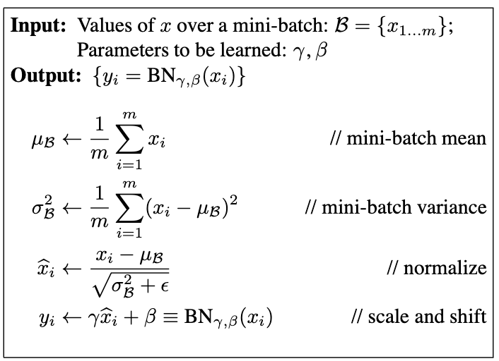
In Stochastic Gradient Descent we train with a mini batch of training data. Batch normalisation consists of normalising the batch in a training iteration. Here are the steps to performing batch normalisation introduced in the paper Batch Normalization: Accelerating Deep Network Training byReducing Internal Covariate Shift
The paper mentioned above introduced the use of Batch Normalisation to improve the performance of neural network training by normalising the batch inputs to address the internal covariant shift. The recent models in Computer vision have been trained with Batch Normalisation and these has resulted in higher accuracies in training and test set. Batch normalisation smoothens the loss which enables training at larger learning rates and larger batch sizes.
However, the effectiveness of Batch Normalisation has been recently also attributed to its ability to smooth the objective function which improves the performance (How Does Batch Normalization Help Optimization?) . However, It does reduce gradient explosion during initiation. (A Mean Field Theory of Batch Normalization)
Batch Normalisation in Keras and TensorFlow
This is how batch normalisation is implemented in Keras
model = keras.models.Sequential([
    keras.layers.Flatten(input_shape=[28, 28]),
    keras.layers.BatchNormalization(),
    keras.layers.Dense(300, activation="relu"),
    keras.layers.BatchNormalization(),
    keras.layers.Dense(100, activation="relu"),
    keras.layers.BatchNormalization(),
    keras.layers.Dense(10, activation="softmax")
])
And in MxNet
net = nn.Sequential()
net.add(nn.Conv2D(6, kernel_size=5),
        BatchNorm(6, num_dims=4),
        nn.Activation('sigmoid'),
        nn.MaxPool2D(pool_size=2, strides=2),
        nn.Conv2D(16, kernel_size=5),
        BatchNorm(16, num_dims=4),
        nn.Activation('sigmoid'),
        nn.MaxPool2D(pool_size=2, strides=2),
        nn.Dense(120),
        BatchNorm(120, num_dims=2),
        nn.Activation('sigmoid'),
        nn.Dense(84),
        BatchNorm(84, num_dims=2),
        nn.Activation('sigmoid'),
        nn.Dense(10))
And PyTorch
net = nn.Sequential(
    nn.Conv2d(1, 6, kernel_size=5), BatchNorm(6, num_dims=4), nn.Sigmoid(),
    nn.MaxPool2d(kernel_size=2, stride=2),
    nn.Conv2d(6, 16, kernel_size=5), BatchNorm(16, num_dims=4), nn.Sigmoid(),
    nn.MaxPool2d(kernel_size=2, stride=2), nn.Flatten(),
    nn.Linear(16*4*4, 120), BatchNorm(120, num_dims=2), nn.Sigmoid(),
    nn.Linear(120, 84), BatchNorm(84, num_dims=2), nn.Sigmoid(),
    nn.Linear(84, 10))
nfnets – High-Performance Large-Scale Image Recognition Without Normalization
Batch Normalisation has three disadvantages :
- It is computationally expensive primitive and has memory overheads.
- It introduces discrepancy in model behaviour between training and inference
- It breaks the independence between training examples in a minibatch
Recent work has used Normalisation free training for ResNets, however to improve performance this paper introduced nfnets. The propose the use of Adaptive Gradient Clipping (AGC). Their smaller models match the test accuracy of an EfficientNet-B7 on ImageNet while being up to 8.7×faster to train, and their largest models attain a new state-of-the-art top-1 accuracy of 86.5%.