Why Distributed Machine Learning?
Contents
In the previous article we looked at how GPGPU, ASICS, AWS’s Inferentia, the new NVidia A100 chip and other advances in hardware have tremendously improved the performance of Machine Learning training and inference. However the increase in the volume of data and the increasing complexity of the machine learning models require that we start training on multiple nodes instead of one. For example, imagine a researcher who wants to build a model from the medical devices attached to the hospital beds. The model would then need to be trained on fine grained data from thousands of beds over months or years. The size of data could run into hundreds of GBs or even TBs. In addition to this, some of the models today have billions of parameters, such as the GPT-3 model from OpenAI.
What’s wrong with training on a single Node?
- The IO requirements for a single node would be too high. If you have a single node processing all the training data, then most of the time would be spent in getting the training batch into the machine.
- The processor may take a long time to converge. Machine Learning is almost always about minimising the loss function and convergence and a single node even with the latest GPGPU would struggle when presented with millions of data points.
- A single node runs the risk of hardware failure and then the training would need to start again, unless you implement smart checkpointing. Checkpointing would then add to the overheard.
- Sometimes it may be economical to use multiple nodes with cheaper hardware compared to one massive node with expensive hardware.
The reasons above indicate that distributed Machine Learning may be the best way forward for training models that have a huge training dataset or a huge model or needs faster results.
However, note that although the effective wall time reduces with Distributed training; the total time taken, if you add time taken by all nodes individually, may actually increase.
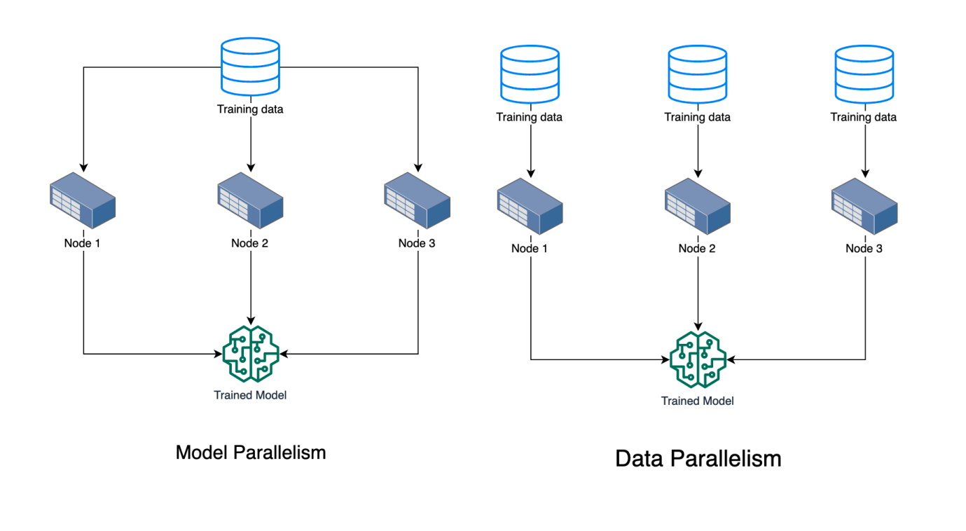
Model Vs Data Parallelism
Model Parallelism
So far we have talked about types of scenarios where distributed training works really well. When we have a huge model that cannot fit into memory, we use distributed ML for “Model Parallelism“. This only works for specific models that can be distributed onto multiple machines. So you have each node working on part of the model and then you combine the results from all nodes to end one iteration.
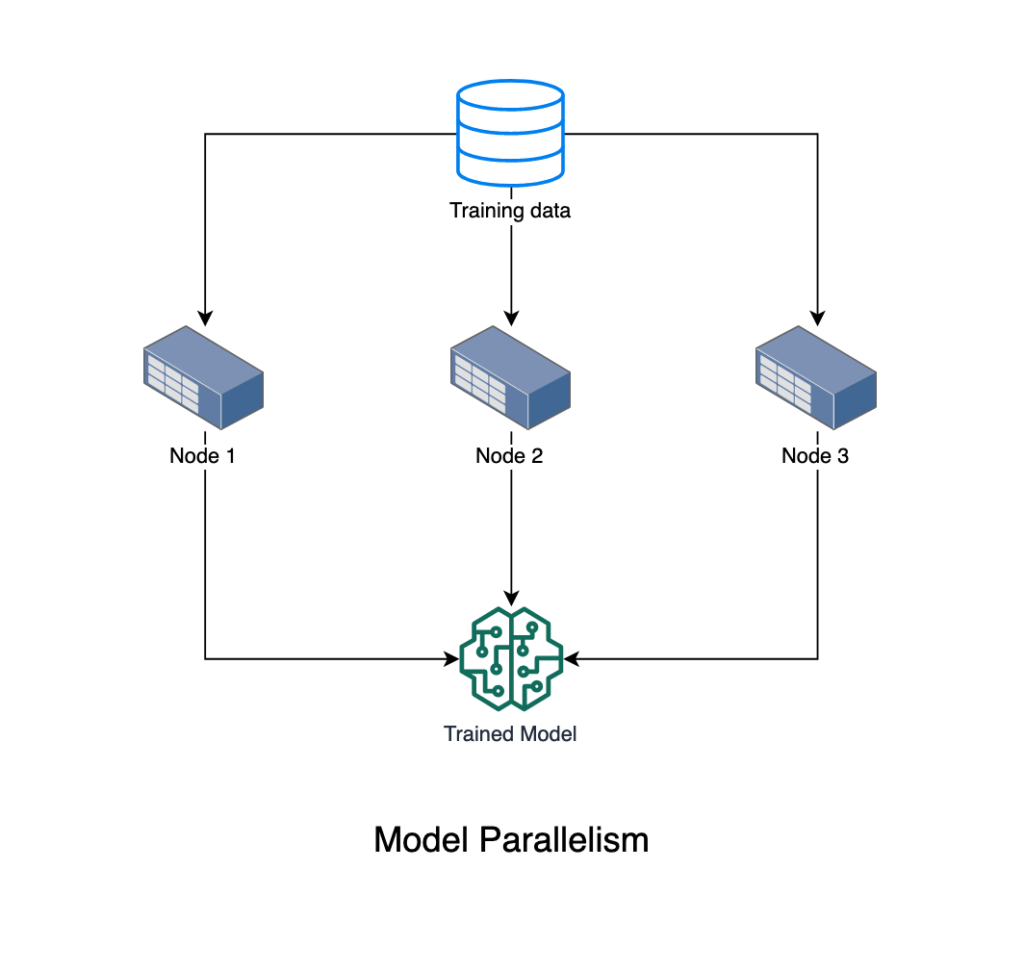
Model Parallelism
Model Splitting
The model needs to be split into multiple nodes and services such as Amazon SageMaker performs automatic model splitting. It performs model splitting based on the framework. For example, for tensorflow it analysis the sizes of training variables and graph structure and uses a graph partitioning algorithm. The model is represented as a directed acyclic graph (DAG) of tf.Operations and therefore the library partitions such that each node for the DAG goes to a device. You can also manually split a model.
Pipeline Execution
Pipelining is a technique that makes the GPUs compute on different data samples and therefore saves time that is lost during sequential computation. Amazon SageMaker splits the batch into smaller microbatches and the microbatches are fed into a pipeline to keep all GPUs busy.
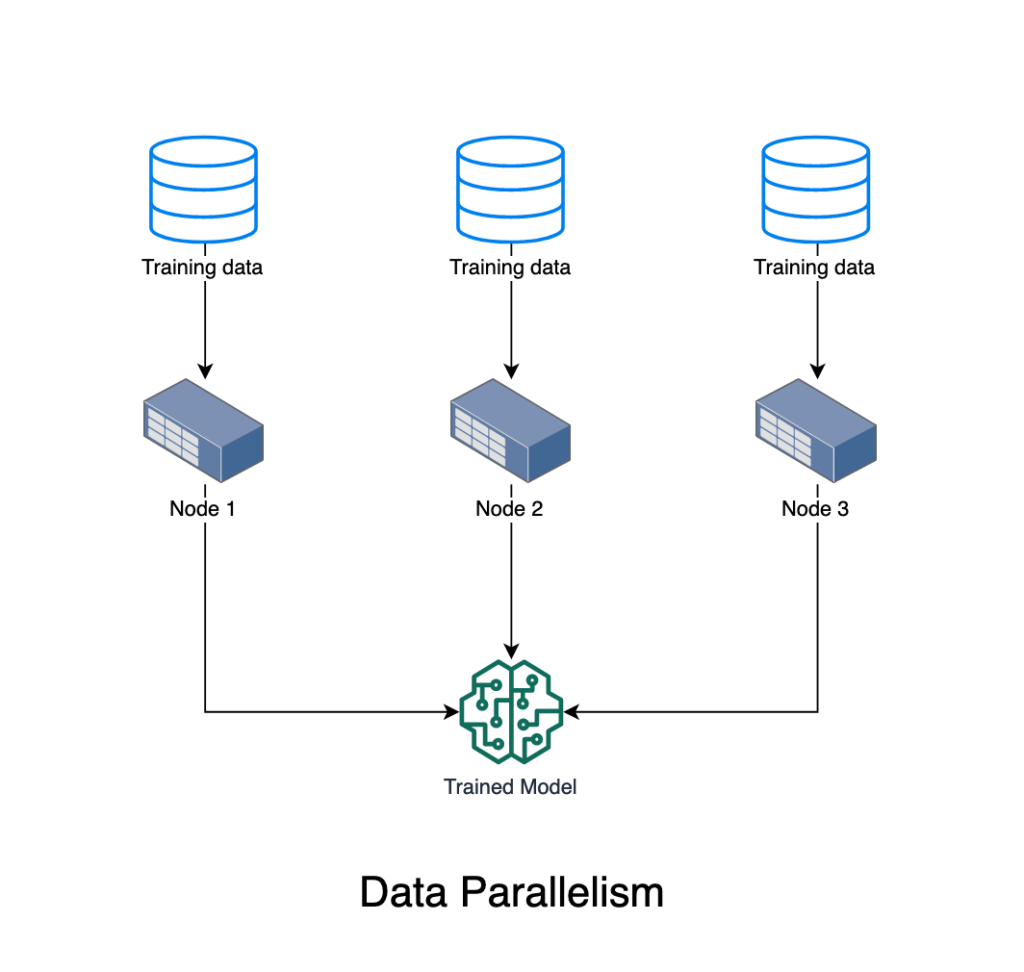
Data Parallelism
In the other case where we have lots of training data, we use a concept called “Data Parallelism” where you distribute chunks of training data to various nodes. Each node has the complete model but only works with part of training data. You then need a way to combine the parameters from each node to go to the next iteration and eventually converge to a solution.
This sounds simple, although there are a few problems that distributed machine learning has to handle. How do the nodes communicate? how are the nodes connected? Lets look at those next.
Communication patterns
Before I describe the topology for distributed learning, it is important to understand how the nodes synchronise the communication with each other. One complication that may arise is that different workers may work at different speeds and hence the partial gradients may not be available from all the workers at the same time. If we use stale gradients during the gradient update phase then convergence may be slower. On the other hand, if you wait for all workers to finish, then it may not be very efficient. There are three models of communication that arise as a result of the tradeoff between speed and convergence.
Bulk Synchronous Parallel (BSP)
The parts of this model are the workers, the communication between them and a barrier. The barrier marks the end of a super step or in our case an iteration. Each worker works on its own gradient and the barrier ensures that the parameter server updates the weights only when it receives the gradient from all the workers. This model tradesoff speed for convergence.
Asynchronous Parallel (ASP)
In this model, all workers send their gradients to the server, but no synchronisation is implemented. Workers do not wait for other workers to complete and hence the parameter server may have stale gradients from a few workers. This causes errors in the gradient calculation and hence delays the convergence. Also, each worker may obtain a different version of weight from the parameter server. Consequently ASP has least training time but yields a lower accuracy and is not stable in terms of model convergence.
Stale Synchronous Parallel (SSP)
This combines ASP and BSP and uses a policy to switch between ASP and BSP dynamically during training. The idea is that the difference in the iteration number for the fastest and the slowest worker should not exceed a user defined number. There is no waiting time, except for the fastest workers that may have to wait for the slowest worker to catch up. The model convergence guarantee is high but decreases as the staleness increases.
We will now look at two different ways to perform the stochastic Gradient descent (SGD) on distributed training data. The first method uses a parameter server and can be thought of as performing Asynchronous SGD while the next method, AllRedue, can be thought of as synchronous SGD.
Parameter server for distributed Machine Learning
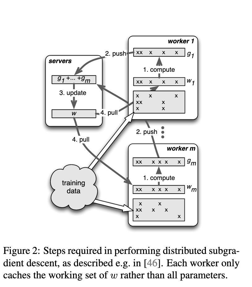
The diagram above sourced from this paper gives an overview of one of the implementations of the parameter server called the distributed subgradient descent. This is how it works – The training data is partitioned amongst the workers. Each worker uses its own training data to calculate a gradient. The gradient is pushed to the Parameter Server. The parameter server combines the gradients from each worker and updates the weights. The weights are then pulled by the workers for the next iteration.
A parameter server can run more than one model training simultaneously.
AllReduce for Distributed Machine Learning
The Second class of algorithms that we will look at belong to the AllReduce type. They are also decentralized algorithms since, unlike parameter server, the parameters are not handled by a central layer. Before we look at the algorithms, lets look at a few concepts
What is MPI and AllReduce?
MPI or Message Passing Interface is a communication protocol standard for passing messages for parallel computing architectures. The standard defines the syntax and rules for libraries for parallel computing. It defines both point-to-point and collective communication protocols.
Collective Functions – broadcast, reduce, allReduce, gather,all-gather, scatter
Collective functions implemented by MPI provide standards for communication between processes in a group. For example the broadcast function takes data from one node and sends it to all the processes (nodes) in the group. The Reduce function collects data from each node and combines them into a global result based on chosen operator. It can be considered an inverse of broadcast. the AllReduce pattern takes the data from each node, performs the reduce operation and sends the data back to all nodes. AllReduce can be thought of as a reduce operation with a subsequent broadcast call. A gather operation stores data from all nodes into a single node. Gather can be thought of as a reduce operation that uses the concatenation operator. AllGather collects data from all units and stores the collected data in all units. Scatter sends data from one node to all the nodes, but unlike broadcast it does not send the same message, but splits the message and sends one part to each node.
Peer to Peer AllReduce
The first AllReduce topology that we look at is the Peer to Peer AllReduce explained in this paper. Here’s a diagram borrowed from that paper
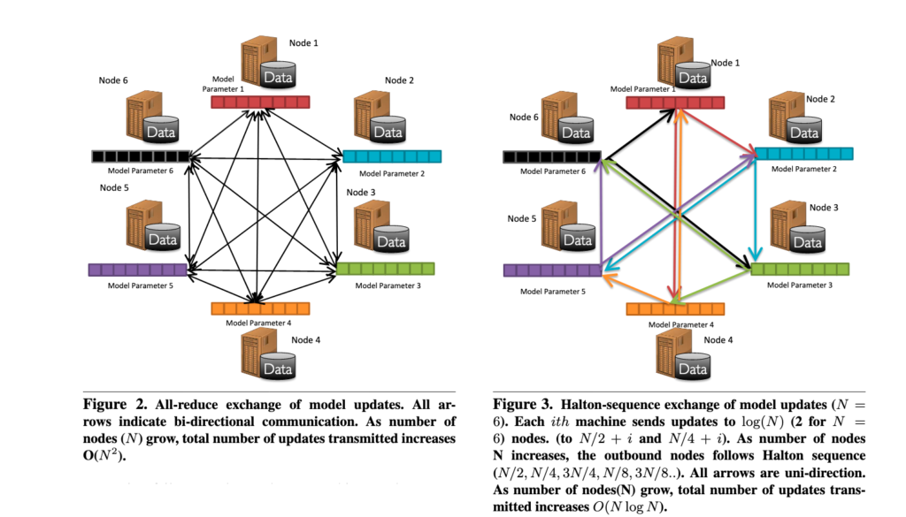
As seen above, the algorithms train in parallel over sharded data. They share model updates after a few iterations. The Model sharing may occur using one of the communication methods described above (BSP, SSP). The advantage with this topology is that there is no central master and hence there is no need for special measures to recover from master failures. Instead of sending data to all peers, its also possible to use allreduce primitives such as butterfly or tree style. However with the tree style. failure of a node is problematic.
Ring AllReduce
The diagram below from the horovod paper shows how the Ring AllReduce works.

A logical ring exists between all the nodes and each node communicates with two adjacent nodes. If the total number of nodes is p, the data is partitioned into p chunks. Each node sends a chunk to a neighbor in the ring and receives a chunk from another neighbor. When it receives a chunk, it performs a reduce operation. This operation is performed p-1 times. This finishes the reduce-scatter operation. Next an AllGather operation is performed in a similar fashion in p-1 steps and that finishes the AllReduce operation. This blog gives a nice visual intuition to the operation.
This is the end of the article for architecture. In the next and last part in the series we will look at software to perform distributed Machine Learning. Stay tuned!
References
Dynamic Stale Synchronous Parallel Distributed Training for Deep Learning
MALT: Distributed Data-Parallelismfor Existing ML Applications
Exhaustive Study of Hierarchical AllReduce Patterns for Large Messages Between GPUs
Horovod: fast and easy distributed deep learning inTensorFlow