Introduction:
In many situations, a relationship between two variables needs to be analysed. For example, a car manufacturer would like to know whether the number of cars bought in the city is related to the average household income in the city, or a sales manager would like to know if the sales revenue is dependent on the discount percentage offered by the company. Such an analysis can be done by Simple Regression. Simple regression involves building a model that can determine one variable given another variable. The known variable is called the independent variable and the variable to be determined is called dependent variable. To do the analysis, the researcher aims to fit the data in a straight line form. i.e. the data is fit into a line of the form y=mx+c; where y is the dependent variable and x is the independent variable. m is slope of line and c is the y intercept. This is also the deterministic model since it gives the exact value of y for a given value of x. Statisticians also use probabilistic models where y can be determined with a given error range.
y=mx+c+e
where e is the error in determination.
For a sample the regression line is given by
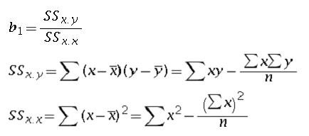
bo and b1 can be obtained for the sample using least square analysis.

Residual Analysis :
Once a regression line is determined, the researcher needs to validate whether the line is a good fit for the data.
To do so, he can use historical information and try to fit this information in the regression line.
For each historical point a residual value is obtained. This is the difference between actual historical value and the value obtained from the regression line. The sum of the squares of this residual values is minimized to find the least squares line. The sum of the residuals is zero for the sample data if there are no rounding errors. A point with high residual value may be an outlier. The residual analysis plot can be used to gauge how effective the regression model is. The residual plot is a plot of the residual value against the independent variable. It checks the following assumptions of simple regression analysis
1) The model is linear
2) The error terms have constant variance, are independent and are normally distributed.
The residual plot can be visually analysed to verify the above assumptions.
Standard Error of estimate:
The standard error of estimate can be used to determine the error that arises out of simple regression. It is the standard deviation of the error terms. the standard error of estimate is given by
Where SSE can be estimated by either of these methods.
The standard error estimate, being the standard deviation value can be used to verify whether the residues are normally distributed. For normal distribution values 68% of values fall within one standard deviation and 95% of values would fall within two standard deviation.
Coefficient of determination :
The coefficient of determination is called r2 (r squared). It is the proportion of variation of the dependent variable(y) explained by the independent variable(x). The value can range from 0 to 1. A value of 0 implies no variation of y w.r.t x and a value of 1 implies all variation in y can be explained by x. From a business point of view, a researcher may chose the value of coefficient to be good or bad depending on the context. A high value is sought by those seeking exact prediction.
The coefficient can be calculated as follows:
the sum of squares of error can be broken into two parts i.e. variance measured by sum of squares of regression(SSR) and sum of squares of error (SSE). The coefficient of determination is given as the proportion of variation explained by regression.
Hypothesis testing for the slope of the regression model:
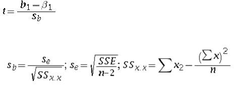
A test to determine whether the regression model is applicable (significant) is to test if the slope of the regression line is significant. The way to do this is to determine if the population mean is different from 0. (If it is different from 0, the variables are related and hence regression model can be applied). A t-test on the slope can be used to determine a null hypothesis of the form .
Null hypothesis – the hypothesized slope is zero.
Alternate hypothesis– the hypothesized slope is greater than or less than zero.
note that this is a two tailed test.
the t test is given by
where beta1=the hypothesized slopes; df = n-2
Confidence interval for the determination of y : y can be determined from x using the regression model. However a confidence interval can be used to determine the range within which the y value falls for that confidence level or the mean of the y value for that confidence level.
The prediction interval for y can be given by:
Note the regression line is obtained from the sample data. This regression line may be valid only for the range of the sample data. Although the regression line is sometimes extrapolated, the results may be incorrect. Hence care should be taken while using the regression model to predict values.
