Continuous values – These can take any values within a specified range. For example height of students in a class can take any value from say 4 feet to 6 feet.
Distribution of discrete variables – lets us first consider the distribution of discrete variables.
Binomial distribution
This is the distribution of results in an experiment where the result can either be a success or a failure. For example a coin toss can be either heads or tails. let p be the probability of success, q be the probability of failure(q=1-p) and n be the number of trials. The probability of x successes is given by
The mean of a binomial distribution is given by (np).
The standard deviation is given by SD=sqrt(npq)
A graph can be plotted by plotting P(x) against x.
Poisson Distribution
This distribution describes the occurrences of rare events. It gives the probability of x occurrences in a specified time interval given that there are lambda expected occurrences in the same time period. for example if it is known that a machine produces 10 defective items in 30 mins, what is the probability that it will produce 4 defective items. The distribution is given by
Binomial problems with large sample sizes and small values of p can be approximated by poisson distribution. Heuristics suggest that if n > 20 and n.p <= 7, then the poisson distribution can be used to approximate binomial distribution.
continuous variables take all values within an interval. To calculate the probability between any two points, find the area under the curve. The total area under the curve for this kinds of distribution is 1. To find the probability at a particular point, the thumb rule is to add and subtract a small quantity and take the area under the two values obtained. i.e. probability at x can be found out by finding area under the curve between the points x+dx and x-dx where dx is around half a unit.
Uniform Distribution – This distribution has a constant value throughout. This is also referred to as rectangular distribution.
The distribution is given by
Image and equation Source – mathworld.wolfram.com.
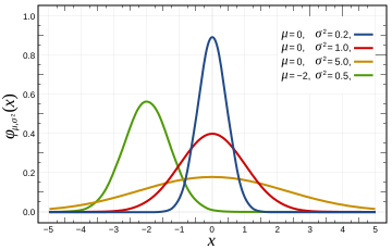
Normal Distribution – This is probably the most frequently encountered distribution and also most widely used. Example of a normal distribution is the error rate of a machining equipment. Physicist refer to it as Gaussian distribution and it is also popularly referred to as a ‘bell curve’.
Image source – Wikepedia
The probability density function is given by
Equation source – mathworld.wolfram.com.
The Normal curve depends on the mean and standard deviation. There would be different curves for each combination of mean and standard deviation, therefore a standardized normal distribution curve is used. This curve is obtained by converting the values of x to its corresponding z score. z score is calculated as (x-mean)/SD.
The z distribution has a mean of 0 and standard deviation of 1. To find the probability between two values in the normal curve, find the area under the curve between the two values. To do so, convert the two values to their corresponding z scores and use the standard z score table to arrive at the associated probability. The difference between the probability of the higher value and the lower values gives the probability for the interval.
The normal distribution can be used as an approximation to the binomial distribution. To do so calculate the mean and SD from n and p using mean = n.p and sd = sqrt(n.p.q). A thumb rule is that the approximation can be applied if mean+3SD lies between 0 and n.
Exponential Distribution : This is similar to Poisson distribution but useful for continuous values. It gives the probability distribution for times between random occurrences. The x values range from 0 to infinity and the curve steadily decreases as x increases.
