Examples using R – Randomized Block Design

Problem : We wish to determine whether or not four different tips produce different readings on a hardness testing machine. An experiment such as these might be part of a gauge capability study. The machine operates by pressingthe tip into a metal test coupon, and frm the depth of the resulting depression, the hardness of the coupon can be determined. THe experimenter has decided to obtain four observations for each tip. There is onlyh one factor – tip type – and a completely randomized single factor deisn would consist of randomly assigning each one of the 4×4=16 runs to an experimental unit, that is , a metal coupon , and observing the hardness reading that results. However, if the metal coupons differ slightly in their hardness, as might happen if they are taken from ingots that are produced in different heats, the experimental units will contribute to the variability observed in the hardness data. As a result the experimental error will reflect both random error and variability between coupons. We would like to remove the variability between coupond from the experimental error. A design that would accomplish this requires the experimenter to test each tip once on each of four coupons. This desin is called a randomized complete block design. Each block contains all the treatments. Within a block the order in which the four tips are tested is randomly determined.
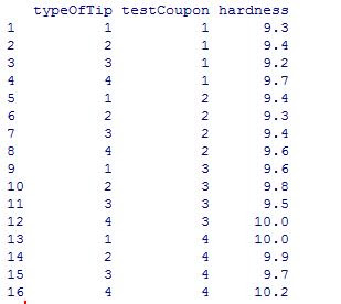
The test data is

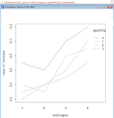
Let us look at the interaction plot

and the box plot

Let us now run the analysis of variance on the data, we will include the blocking variable in the analysis.
the formula to be used in R is hardness~typeOfTip+testCoupon.

> anova(aov(hardness~factor(typeOfTip)+factor(testCoupon)))
Analysis of Variance Table

Signif. codes: 0 ‘***’ 0.001 ‘**’ 0.01 ‘*’ 0.05 ‘.’ 0.1 ‘ ’ 1

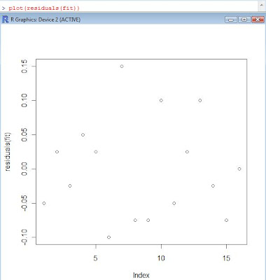
A plot of the residuals should not show any pattern since the residuals are assumed to be independently distributed for analysis of variance. Here’s the plot of the residuals.

A Quantil-Quantile plot can be used to check the distribution as well. The plot also shows the presence of outliers, if any. The plot is shown below.

Tukeys test can be used for pairwise comparison. Here’s the result of the Tukey’s test
fit=aov(hardness~factor(typeOfTip)+factor(testCoupon))
TukeyHSD(fit,which=’factor(typeOfTip)’,ordered=”TRUE”)

A plot of the residuals should not have a pattern. Here’s a plot of the residuals.

We can check for variance. Here’s a method to check to equality of variance.
> summary(lm(abs(fit$res)~typeOfTip))

Call:
lm(formula = abs(fit$res) ~ typeOfTip)

Residuals:
Min 1Q Median 3Q Max
-0.050000 -0.032812 -0.003125 0.026562 0.093750

Coefficients:
Estimate Std. Error t value Pr(>t)
(Intercept) 0.075000 0.024719 3.034 0.00893 **
typeOfTip -0.006250 0.009026 -0.692 0.50000
—
Signif. codes: 0 ‘***’ 0.001 ‘**’ 0.01 ‘*’ 0.05 ‘.’ 0.1 ‘ ’ 1

Residual standard error: 0.04037 on 14 degrees of freedom
Multiple R-squared: 0.03311, Adjusted R-squared: -0.03595
F-statistic: 0.4795 on 1 and 14 DF, p-value: 0.5

Since the p-value is large, difference in variance cannot be stated.

The Latin Square Design:
If there are two blocking variables then the latin square design can be used.
problem : Suppose that an experimenter is studying the effects of five different formulations of a rocket propellant used in aircrew escape systems on the observed burning rate. Each formulation is mixed from a batch of raw material that is only large enough for five formulations to be tested. Furthermore, the formulations are prepared by several operators, and there may be substantial differences in the skills and experience of the operators.
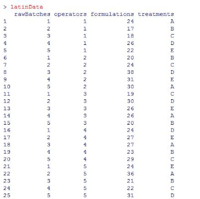
Here’s the data

The latin square structure is
> matrix(treatments,5,5)
[,1] [,2] [,3] [,4] [,5]
[1,] “A” “B” “C” “D” “E”
[2,] “B” “C” “D” “E” “A”
[3,] “C” “D” “E” “A” “B”
[4,] “D” “E” “A” “B” “C”
[5,] “E” “A” “B” “C” “D”

An analysis of variance gives
> anova(lm(formulations~factor(rawBatches)+factor(treatments)+factor(operators)))

The data shows that the different formulations do produce different burning rate. Also there is a difference between the operators. However, no difference between the raw batches.